When I saw oscilloscope music demos, they amazed and inspired me.

Observing a clever use of interaction between sound and an electron beam is a unique experience.

Some awesome oscilloscope music videos: Youscope, Oscillofun and Khrậng.

However, I could not find any beautiful oscilloscope emulators. Lines produced by most emulators barely look like real oscilloscope lines at all.

Because of that I made a cool WebGL demo — woscope, which is a XY mode oscilloscope emulator.

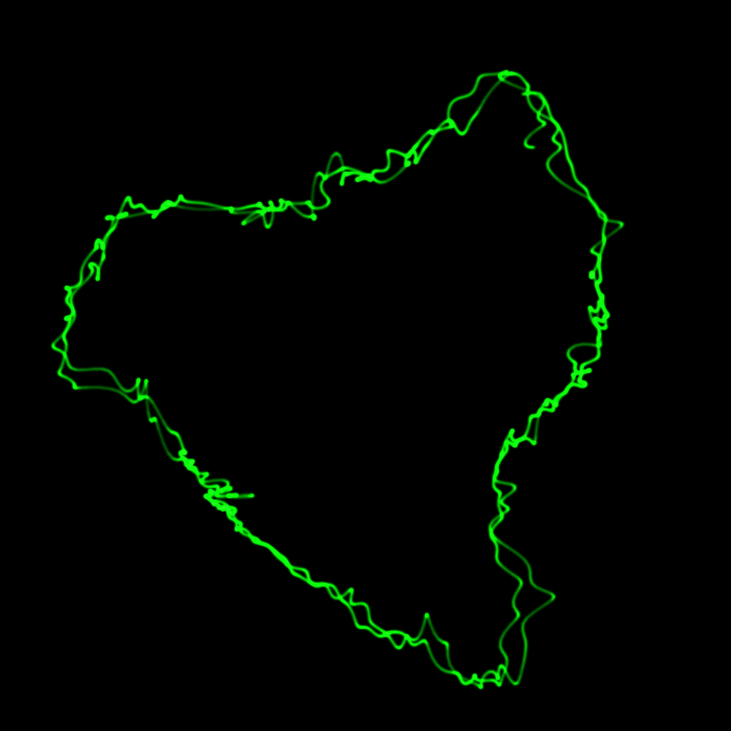
In this post you can learn how to draw these lines in WebGL.

Problem formulation

We have a stereo sound file. We want to draw a line that looks like oscilloscope line, when the oscilloscope is connected in XY mode.

Each pair of samples from the sound file interpreted as 2D point.

I decided to draw each line segment by drawing a rectangle that affected by electron beam moving from the start to the end of the segment.

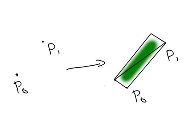
This has two interesting implications:

• There is no corner case for segment joints
• There will be triangle overdraw, which might cause loss of performance

Beam intensity is collected from different segments using blendFunc(gl.SRC_ALPHA, gl.ONE);.

Generating vertices

For a line segment, for each point of a rect we calculate vertices position using segment start point, segment end point and index of the vertex.

it might be weird to store the same point 4 times in a buffer, but I could not find a better way

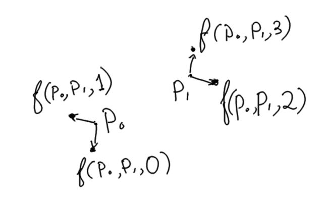
The forst two points are close to the starting point, second two points are close to the ending point. Even points are shifted to the “right” of the segment and odd point are shifted to the “left” of the segment.

This transformations is pretty straightforward in glsl:

#define EPS 1E-6
uniform float uInvert;
uniform float uSize;
attribute vec2 aStart, aEnd;
attribute float aIdx;
// uvl.xy is used later in fragment shader
varying vec4 uvl;
varying float vLen;
void main () {
    float tang;
    vec2 current;
    // All points in quad contain the same data:
    // segment start point and segment end point.
    // We determine point position using its index.
    float idx = mod(aIdx,4.0);

    // `dir` vector is storing the normalized difference
    // between end and start
    vec2 dir = aEnd-aStart;
    uvl.z = length(dir);

    if (uvl.z > EPS) {
        dir = dir / uvl.z;
    } else {
    // If the segment is too short, just draw a square
        dir = vec2(1.0, 0.0);
    }
    // norm stores direction normal to the segment difference
    vec2 norm = vec2(-dir.y, dir.x);

    // `tang` corresponds to shift "forward" or "backward"
    if (idx >= 2.0) {
        current = aEnd;
        tang = 1.0;
        uvl.x = -uSize;
    } else {
        current = aStart;
        tang = -1.0;
        uvl.x = uvl.z + uSize;
    }
    // `side` corresponds to shift to the "right" or "left"
    float side = (mod(idx, 2.0)-0.5)*2.0;
    uvl.y = side * uSize;
    uvl.w = floor(aIdx / 4.0 + 0.5);

    gl_Position = vec4((current+(tang*dir+norm*side)*uSize)*uInvert,0.0,1.0);
}

Calculating the intensity with math

Now that we know where to draw a quad, we need to calculate the cumulative intensity at any given point in the quad.

Let’s assume that electron beam has gaussian distribution, which is not that uncommon in physics.

Where σ is the spread of the beam.

To calculate the cumulative intensity, we integrate the intensity over time as the beam is moving from start to end.

If we use the frame of reference where start point is at $(0,0)$ and the end point is $(length,0)$, $distance(t)$ can be written as:

Now,

Since $p_y^2$ is a constant in this integral, $e^{-\frac{p_y^2}{2σ^2}}$ can be taken out of the integration.

Let’s simplify the integral slightly, by replacing $t$ with $\frac{u}{l}$:

The integral of normal distribution is half error function. w|a

Finally,

One of the benefits of doing math in this case is that segment joints will have mathematically perfect intensity after adding adjacent segments.

The resulting formula is not hard to implement in framgent shader in glsl.

Fragment shader

The uvl varying in the vertex shader contains coordinates in which start point is $(0,0)$ and end point is $(length,0)$.

Since varyings are interpolated linearly for the fragment shader, we get the point coordinates in required frame of reference for free.

The rest is writing the math formula in glsl, and handle a corner case when the length of the segment is too small.

gaussian function and erf approximation for glsl is shamelessly stolen from Evan Wallace’s blog

#define EPS 1E-6
#define TAU 6.283185307179586
#define TAUR 2.5066282746310002
#define SQRT2 1.4142135623730951
uniform float uSize;
uniform float uIntensity;
precision highp float;
varying vec4 uvl;

// A standard gaussian function, used for weighting samples
float gaussian(float x, float sigma) {
  return exp(-(x * x) / (2.0 * sigma * sigma)) / (TAUR * sigma);
}

// This approximates the error function, needed for the gaussian integral
float erf(float x) {
  float s = sign(x), a = abs(x);
  x = 1.0 + (0.278393 + (0.230389 + 0.078108 * (a * a)) * a) * a;
  x *= x;
  return s - s / (x * x);
}

void main (void)
{
    float len = uvl.z;
    vec2 xy = uvl.xy;
    float alpha;

    float sigma = uSize/4.0;
    if (len < EPS) {
    // If the beam segment is too short, just calculate intensity at the position.
        alpha = exp(-pow(length(xy),2.0)/(2.0*sigma*sigma))/2.0/sqrt(uSize);
    } else {
    // Otherwise, use analytical integral for accumulated intensity.
        alpha = erf(xy.x/SQRT2/sigma) - erf((xy.x-len)/SQRT2/sigma);
        alpha *= exp(-xy.y*xy.y/(2.0*sigma*sigma))/2.0/len*uSize;
    }

    float afterglow = smoothstep(0.0, 0.33, uvl.w/2048.0);
    alpha *= afterglow * uIntensity;
    gl_FragColor = vec4(1./32., 1.0, 1./32., alpha);
}

Things that can be improved

The resulting picture looks pretty nice, however there are several problems with current implementation.

• The electron beam should not move in straight lines between sample points. There are no sharp corners on a real oscilloscope, but sometimes there are sharp corners in the current implementation.
  It would probably be benefitial to implement a sinc interpolation to increase the number of points.

• Point intensity is saturated too fast. I’ve added a workaround by giving little red and blue value to the color, so oversaturated pixels look white.

• No account for gamma correction.

• There is no post-processing bloom, but is it really required?

• Currently, woscope is a PoC of this technique, should it be implemented as JavaScript library?

• Implement the oscilloscope emulator as a native program?

Summary

Using math is extremely beneficial when emulating physical processes.

I’ve never seen an oscilloscope beam implemented this way, and I really like the resulting picture. This technique can be used to draw other soft lines.

I hope this will help people drawing beautiful lines using WebGL/OpenGL :)

code on this page is in Public Domain, except erf and gaussian functions borrowed from other blog